Community Banking Connections

Print Article

Essentials of Effective Interest Rate Risk Measurement
by Emily Greenwald, Assistant Vice President, Federal Reserve Bank of Chicago and Doug Gray, Managing Examiner, Federal Reserve Bank of Kansas City

Interest rate risk (IRR) is defined as the potential for changing market interest rates to adversely affect a bank's earnings or capital protection. Two previous issues of Community Banking Connections included articles on IRR management for community banks.¹ The first article provided an overview of key elements of an IRR management program and common pitfalls faced at community banks. The second article focused more attention on directors' and senior managers' specific responsibilities, including development of sound policies and IRR exposure limits. In this article, the discussion proceeds to IRR measurement issues, including the appropriateness of certain measures and some of the challenges faced in modeling risk exposures.

Perhaps the most discussed IRR management topic for community banks is risk measurement. Community bankers often ask which techniques, tools, and models are needed and how those tools can be fine-tuned. At the most basic level, regulators expect a bank's IRR measurement tools and techniques to be sufficient to quantify the bank's risk exposure. ²

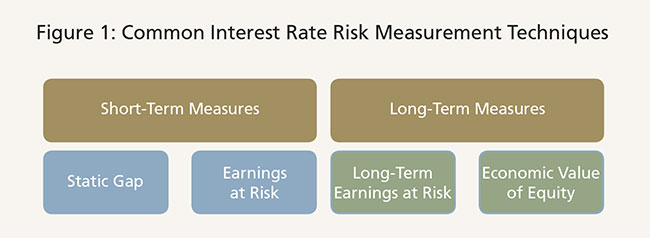
Measurement techniques typically fall into two broad categories: short-term and long-term risk measures (Figure 1). Generally speaking, short-term measurement techniques attempt to quantify the size of a bank's risk relative to the earnings stream generated by bank operations. Alternatively, long-term measurement techniques attempt to quantify the size of a bank's risk relative to its capital protection.

Measuring IRR is nothing new, as bankers have measured aspects of IRR for decades beginning with basic static gap analyses. Technological advancements have allowed IRR measurements to evolve from simple spreadsheet calculations to software and third-party vendors capable of measuring complex cash flows. Today, even noncomplex community banks can obtain cost-effective asset/liability management (ALM) models to quantify both short-term and long-term IRR exposures (although the Federal Reserve does not require community banks to purchase such models). While some of these models use complex mathematical computations to calculate a bank's IRR exposure, the short- and long-term measures captured by these ALM models are conceptually straightforward. Before discussing essential considerations in selecting and operating an ALM model, it is important to clearly understand each measure conceptually.

Short-Term Measures

Short-term measurement techniques quantify the potential reduction in earnings that might result from changing interest rates over a 12- to 24-month time horizon. The two most common short-term measures for community banks are static gap reports and earnings-at-risk (EaR) analysis.

Static Gap

Static gap reports attempt to highlight potential "gaps" in the near future (typically over the next 12 months), where changes to interest rates on assets such as loans and bonds, or liabilities such as deposits, do not occur contemporaneously. Thus, when the prevailing market interest rates change, a bank could experience net interest margin compression, reduced net income, or both. Assets and liabilities with interest rates that change in the measurement window (say 12 months) are referred to as "rate-sensitive." The difference between cumulative rate-sensitive assets and liabilities for the period being measured is referred to as the "static gap." A large gap indicates a potentially significant IRR exposure. For example, a bank with rate-sensitive assets that significantly exceed the volume of rate-sensitive liabilities would expect the net interest margin to decline when market interest rates also decline. While the static gap report might provide some indication of the direction of IRR, it is an imprecise risk measurement tool. Specifically, the static gap report does not effectively capture cash flow timing from unscheduled loan and bond payments (prepayments), and slotting the repricing horizon of nonmaturity deposits becomes extremely difficult at best. Thus, it may only be suitable for banks that have very low IRR profiles to rely solely on this measure to quantify short-term IRR exposures.

Earnings at Risk (EaR)

Because of the shortcomings of static gap reports, most community banks have implemented IRR models that compute EaR over a 12-month or 24-month time horizon to quantify short-term earnings exposures. To compute these earnings exposures, most models begin by calculating either net interest income or net income in a scenario in which interest rates do not change (base case). Income and expenses are then recalculated in scenarios with higher and lower interest rates. The results of each variation are compared against the base case scenario to determine the potential change in earnings from each.

Long-Term Measures

Long-term measurement techniques quantify the potential exposure to capital — either through reduced long-term earnings or a reduced economic value of capital — that might result from changing interest rates. While long-term (up to five years) net income simulations (i.e., EaR analysis) are occasionally used at community banks, the most common long-term measurement technique is some variation of economic value of equity (EVE) analysis. EVE analysis, unlike the EaR measure, involves projecting cash flows from assets and liabilities over the economic life of each product, assuming interest rates will not change. Cash flows are then discounted to determine their present value, and the present value of liabilities is subtracted from the present value of assets to determine the bank's EVE in a base case. Cash flows are also projected for various rising and falling interest rate scenarios and discounted at higher and lower discount rates to recalculate the EVE. The percent change in EVE from the various scenarios provides a meaningful measure of the bank's long-term IRR exposure relative to capital. The real value in EVE analysis is identifying risk exposures that extend beyond the next 12 to 24 months. For example, if a bank's analysis reflects a significant reduction in EVE in a period of rising rates, research has indicated that the bank's financial performance would be expected to deteriorate in the years following a period of increasing interest rates. ³

It is a longstanding expectation by U.S. banking supervisors that all banks will assess the potential impact of IRR on earnings and capital. While EVE analysis is a beneficial measure of long-term IRR exposure for community banks, regulatory guidance does not require every community bank to conduct such analysis. EVE analysis is particularly useful, and often required by examiners, for banks with long-term bond portfolios and assets with embedded options. The risks from these assets are typically not captured by short-term measures. Community banks with short-term balance-sheet structures and ample capital and earnings, however, would not always be expected to use EVE analysis to compute long-term IRR exposures.

Key Considerations

When a bank considers purchasing ALM model software or contracting with a third party to measure its IRR, a number of considerations should factor into the decision. Some of these considerations include, but are not limited to, the intended use of the model, cost, measurement capabilities, features, reporting, and customer support. When selecting any ALM model, management should also weigh the strengths of the model against its limitations. Choosing an ALM model is a bank-specific decision, where one size truly does not fit all. From a regulatory perspective, we will focus on two key considerations: a bank's intended use and the measurement capabilities of the model.

Intended Use

Evaluating management's intended use is a key first step in selecting an ALM model. An important primary use of any bank's ALM model is measuring the bank's IRR exposure. While this seems intuitive, not all community bankers have given the appropriate consideration to measuring all of the bank's material IRR exposures. Once established, the ALM model may also be used for other purposes, such as profit planning, asset pricing, liquidity planning, and other functions, all of which are distinct and secondary to basic IRR measurement.

As discussed earlier, ALM model results are derived by projecting cash flows, which contemplate likely behavior of the bank's management team and customers to changing market interest rates. The simplest ALM models create cash flows and accrual calculations from Call Report data fields, while more sophisticated models derive such information from detailed product attributes of the bank's assets and liabilities. By projecting these cash flows, ALM models are used to construct commonly utilized EaR and EVE measures. Since the primary intended use is measuring EaR and EVE, understanding the capabilities and key assumptions that go into these calculations is crucial to evaluating an ALM model.

Measurement Capabilities

Another key consideration in choosing the appropriate ALM model is the measurement capabilities of the software or third-party vendor. Some models provide the user with a standard set of basic interest rate change scenarios, such as instantaneous, uniform changes in all prevailing market rates (for example, all rates increase 300 basis points) that are evaluated against the existing balance sheet. Other models provide the ability to evaluate the effects of nonparallel interest rate changes (for example, short-term rates increase, while long-term rates remain stable), delayed reactions to rate changes (for example, certificate of deposit (CD) rate changes 90 days after prevailing market rate changes), and balance-sheet changes that may result from market rate changes (referred to as "dynamic" balance-sheet modeling). Guidance from federal and state banking regulators in 2010 (with subsequent frequently asked questions in 2012 to clarify the 2010 guidance) emphasized the importance of evaluating the ALM model's measurement capabilities against material products and services on the bank's balance sheet.⁴

A couple of examples might be helpful in clarifying the guidance in this area. First, consider a bank that is exposed to basis risk because the rates that drive asset pricing differ from the rates that drive liability pricing. This bank has a large volume of loans priced off of national prime rates, which are funded by three-month CDs priced off of U.S. Treasury bill rates. To quantify this IRR exposure, management would need to ensure that the ALM model is capable of evaluating changes to more than one key market rate.

Another example that has become more prominent in recent years is a bank that originates and sells mortgage loans but retains the servicing rights. Some ALM models only measure changes to net interest income (NII) rather than potential changes to all income and expense categories. Since fee income from mortgage originations and ongoing servicing fees are sensitive to interest rates, calculating the change in NII would fail to capture the fee income at risk in various rate environments. Banks with significant noninterest income that is sensitive to changing rates should focus special attention on quantifying potential changes to net income. A bank should ensure that its ALM model is capable of quantifying the effect that market rate variations could indirectly have on its earnings.

More broadly, a bank should also understand the benefits and limitations in the level of detail for which assets and liabilities are analyzed in the model. A model that is based upon Call Report schedules may be appropriate for lower-risk banks with homogeneous loan and security characteristics. While these ALM models are often less expensive and more easily implemented and operated, grouping assets and liabilities in the model based upon Call Report categorization also has a downside. For example, Call Report instructions define any loan operating at or below an interest rate floor as a fixed-rate loan. ALM models using this categorization of assets would also treat these otherwise variable-rate loans as fixed-rate loans and miscalculate the contribution of these assets to earnings in various interest rate change scenarios. Call Report-based models have similar limitations for other loan and deposit features as well, lessening their accuracy as a risk measurement tool. Thus, an ALM model's material limitations should be clearly understood by the ALM committee or board of directors when reviewing ALM model reports.

Questions to consider when reviewing the measurement capabilities of an ALM model include:

• How much flexibility does the bank have to set and/or modify the interest rate scenarios employed in the ALM model?
• How frequently can the ALM model be run and the results be made available to the bank?
• Can the level of asset and liability detail be customized, or is the model limited to Call Report fields?
• Can the ALM model measure nonparallel interest rate scenarios? If so, how much input does the bank have in determining the scenario(s) to run?
• Does the model measure key risks, such as basis, mismatch, prepayment, and yield curve risks? If not, are any of these risks material to the balance sheet?

ALM Model Assumptions

An effective IRR measurement tool is expected to have an appropriate degree of precision, which depends upon properly established assumptions. While regulators do not expect an ALM model to predict the future, the data used in the tool should have a high degree of accuracy. If data inputs or model assumptions are invalid or inaccurate, the model output reports will not be very useful and could result in poor decisions being made. Likewise, if the reports do not provide meaningful information, they could be ignored by management. As community bank examiners have reviewed ALM models over the past 15 years, they have found that two common assumptions significantly impact the accuracy of model results - deposit behaviors and prepayments. In fact, slight errors in these assumptions can result in significant errors in ALM model results.

Deposit Assumptions

Deposit products continue to represent the most significant funding source for community banks, making deposit assumptions critical to ALM model accuracy. While a bank holds the option to set deposit rates for NMDs and other deposit products like CDs, consumers hold the option to withdraw funds at will. Consequently, assumptions like deposit betas and deposit average lives play a vital role in a bank's measurement system. (See box above for descriptions of deposit beta and deposit average life.)

Most ALM models provide a bank with the flexibility to customize deposit betas. However, not all ALM models provide the ability to input different deposit betas for rising and falling rate scenarios. Deposit betas indirectly affect projected interest expenses under various interest rate change scenarios. In most situations, banks delay raising or lowering deposit rates at the beginning of a rate cycle. When a bank finally elects to change deposit rates, it often will do so to a lesser extent than the prevailing change in market interest rates and often to different degrees depending on whether the rate change is upward or downward. Thus, setting deposit beta assumptions is challenging, as bankers must balance controlling interest expense with customers' ability to transfer accounts.

An ALM model's deposit assumptions also include setting deposit average lives. Assumptions made about the average life of NMDs often have a critical effect on model calculations of EVE. Risk managers should explore how an ALM model enables deposit average life information (sometimes entered as a rate of decay to the balance) to be input. Many community banks turn to vendor-supplied deposit assumptions as a starting point or source for setting the average life for NMD products. Bank management should evaluate how any vendor-supplied assumptions in the model, such as deposit decay rate tables, are updated and maintained by the vendor and compare them with their customers' behavior.

In today's environment, deposit volumes at community banks are at high levels relative to total liabilities. Many community banks have also experienced migration of customer balances from CDs into NMDs since 2008. This influx of NMDs makes sensitivity testing of ALM model assumptions valuable to a community bank. Sensitivity testing takes one key assumption, such as deposit betas, and changes the value to be larger or smaller than its current value. The model scenarios are then run again to see what impact changing one assumption has on the overall ALM model results. Another approach to sensitivity testing is to reallocate a portion of NMD balances into CDs. By measuring traditional deposit mix balances, a bank can be informed of possible outcomes should funds revert back to a more traditional NMD/CD deposit mix that prevailed before 2008.

Questions to consider regarding an ALM model's deposit assumption capabilities include:

• Does the ALM model break out NMDs and CDs beyond the Call Report categories? If the ALM model is Call Report-based, how does customer behavior compare with characteristics of deposits grouped together?
• Does the model allow for different deposit betas in rising and falling rate scenarios?
• How does the model handle deposit average lives? If default assumptions are provided, how are they generated? Can the bank alter default assumptions to reflect customer behavior?
• Does the model allow sensitivity testing of deposit betas and decay rates?
• Does the model enable the deposit product mix to be altered for sensitivity testing purposes?

Prepayment Assumptions

Typically, one of the most difficult IRR measurement challenges is modeling cash flows for mortgages and mortgage-related products. For example, the uncertainty of expected cash flow timing and amounts for products such as residential mortgages, mortgage-backed securities (MBS), and collateralized mortgage obligations (CMOs) depends on the embedded option held by each underlying borrower to refinance or prepay. During periods of low and/or decreasing interest rates, similar to the current environment, the incentive for borrowers to refinance their mortgage is greater and, as such, their propensity to prepay increases. Conversely, during periods of increasing rates, this incentive diminishes and prepayments are likely to be lower. 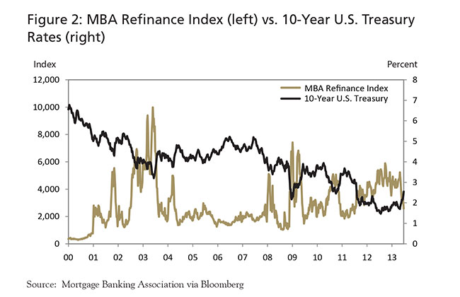Volatile mortgage refinancing cycles over the past decade, however, have not followed traditional theory, which further emphasizes the difficulty in developing prepayment assumptions. Figure 2 illustrates the Mortgage Banking Association's Refinance Index level and the 10-year constant maturity Treasury (CMT) rate between January 2000 and January 2013. As illustrated, homeowners' refinancing activities have not always behaved as expected during periods of interest rate changes, which causes difficulties in estimating future cash flows and potentially leads to erroneous IRR model results. For example, in 2009, 10-year Treasury rates increased after a brief period of low rates. Normal expectations would be that refinancing activity would decline. However, the opposite actually occurred. Other factors, such as government programs, were influencing prepayments during that period.

For banks with material volumes of mortgage-related products, understanding the ALM model's incorporation of prepayment assumptions is essential. ALM model vendors offer an array of prepayment measurement capabilities, from a single prepayment speed for all products to different prepayment speeds for assorted products based on various factors. With respect to modeling mortgages and mortgage-related products, factors such as loan size, seasonality, age of the loan, home sale rates, and loan-to-value percentages may be used to derive prepayment measures and model assumptions.

As with deposit assumptions, value may be found in sensitivity testing prepayment assumptions to determine the risk that earnings may be reduced by elevated prepayments or that EVE may be reduced by slower prepayments. In considering an ALM model, banks should explore the ability and ease of changing prepayment assumptions. With some models, the ability to implement and customize prepayment assumptions requires add-on features, which often adds expense. Regulators would expect that banks having a material amount of mortgage-related or other amortizing assets would incorporate these add-on ALM model features. For these banks, an ALM model that does not effectively incorporate prepayments or resolve the difficulties in estimating future cash flows is likely to produce results that do not adequately quantify the bank's actual IRR exposure.

Bankers often rely on vendors or modeling software providers to provide prepayment assumptions. Regardless of the method used to derive these assumptions, the ultimate goal should be to capture the risk to earnings and capital created by unexpected changes to projected cash flows. Questions to consider when evaluating an ALM model's prepayment assumption capabilities include:

• How does the ALM model incorporate prepayment assumptions?
• Does the ALM model allow prepayment speeds to be assigned for each product?
• Does the model provide default prepayment options? If default assumptions are provided, does the vendor explain how they are generated?
• How reasonable are the prepayment assumptions provided?
• Does management have the ability to alter default assumptions to reflect customer behavior?

In closing, not all ALM models provide the same functionality or produce the same results. The forward-looking nature of IRR measurement techniques presents challenges even for sophisticated ALM models. A bank should select an ALM solution that reliably and cost-effectively delivers the necessary functions for the bank's activities and risk profile. This discussion has provided several considerations and questions that should be useful in evaluating a bank's IRR measurement practices. As additional ALM questions arise, banks should not hesitate to contact supervisory staff at their local Reserve Bank.